Here’s a pretty cool article on understanding PyTorch conv1d shapes for text classification.
In this article, the shape of the example is:
n = 1: number of batchesd = 3: dimension of the word embeddingl = 5: length of the sentence
import torch.nn as nn
import torch

# Example represents one sentence here
example = torch.rand(n=1, l=3, d=5)
example.shape # torch.Size([1, 5, 3])
example

# This is the output:
tensor([[[0.0959, 0.1674, 0.1259],
         [0.8330, 0.5789, 0.2141],
         [0.3774, 0.8055, 0.4218],
         [0.1992, 0.4722, 0.3167],
         [0.4633, 0.0352, 0.8803]]])
In the above output, you can image each row represents one word.
To make the tensor fit into a conv1 layer, we need to reshape it to have the channel first:
# Batch size remains the same
# Use permute() to move the channel first:
example = example.permute(0,2,1)
example

# This is the output:
tensor([[[0.6075, 0.4998, 0.4491, 0.6581, 0.4392],
         [0.2709, 0.1681, 0.5006, 0.3150, 0.8715],
         [0.4999, 0.2203, 0.8735, 0.9370, 0.4723]]])
With the new shape, you can think of the new structure as an image, and each row is one channel of an image: R, B, G.
In terms of a sentence, you can think of it as different semantic spaces of the same sentence. In the blog post that I linked above, the example sentence the author uses is word embedding is so cool.
Now let’s define a conv1d layer:
conv1 = nn.Conv1d(d, 1, 2)
where:
- input channel = 3, the same as the word embedding dimension
- output channel = 1, in this case, the classification label
- kernel size = 2
- stride = 1, this is the default value
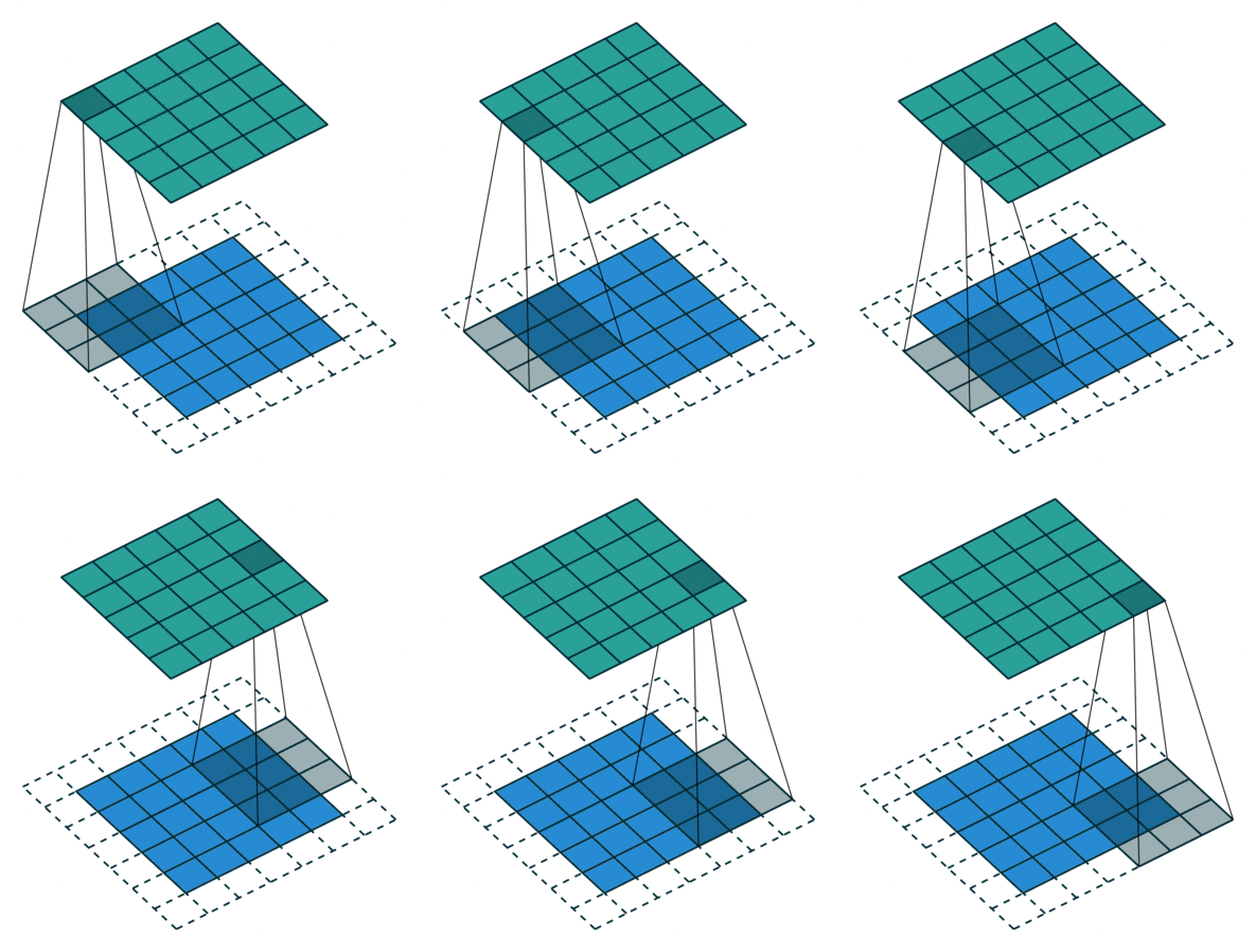
The kernel size defines the field of view of convolution. A common choice of kernel size is 3, and that means $3x3$ pixels.
Here’s a visualization that I got from this blog post: An Introduction to different Types of Convolutions in Deep Learning:

In our case, when kernel size is set to 2, that means we operate on 2 words at a time. Again, given the example word embedding is so cool in the blog post:
- [
word,embedding] -> value - [
embedding,is] -> value - [
is,so] -> value - [
so,cool] -> value
Let’s run the math in my case:
example
# the example:
tensor([[[0.6075, 0.4998, 0.4491, 0.6581, 0.4392],
         [0.2709, 0.1681, 0.5006, 0.3150, 0.8715],
         [0.4999, 0.2203, 0.8735, 0.9370, 0.4723]]])

conv1.weight
# the weight matrix:
tensor([[[ 0.2121,  0.3245],
         [ 0.3465, -0.0467],
         [-0.0528,  0.0373]]], requires_grad=True)

conv1.bias
# the bias term:
tensor([-0.0737], requires_grad=True)
Let’s calcualte the convolution value of [word, embedding]:
The embedding values are:
# word:
[[[0.6075,
   0.2709,
   0.4999]]]

# embedding:
[[[0.4998,
   0.1681,
   0.2203]]]
The result should be:
# "word" * weight
(0.6075 * 0.2121) + (0.2709 * 0.3465) + (0.4999 * -0.0528)

# "embedding" * weight
+ (0.4998 * 0.3245) + (0.1681 * -0.0467) + (0.2203 * 0.0373)

# bias term
+ (-0.0737)

= 0.2851749
If I run the example through the conv1d example:
output = conv1(example)

# Output
tensor([[[0.2852, 0.2338, 0.3826, 0.2449]]], grad_fn=<ConvolutionBackward0>)
As you can see, the first convolution value is 0.2852.
For more detail, check out the blog post that I mentioned above.