Introduction
In this blog, I will talk about the model part for assignment 2 of XCS300. Here’s the link to the assignment.
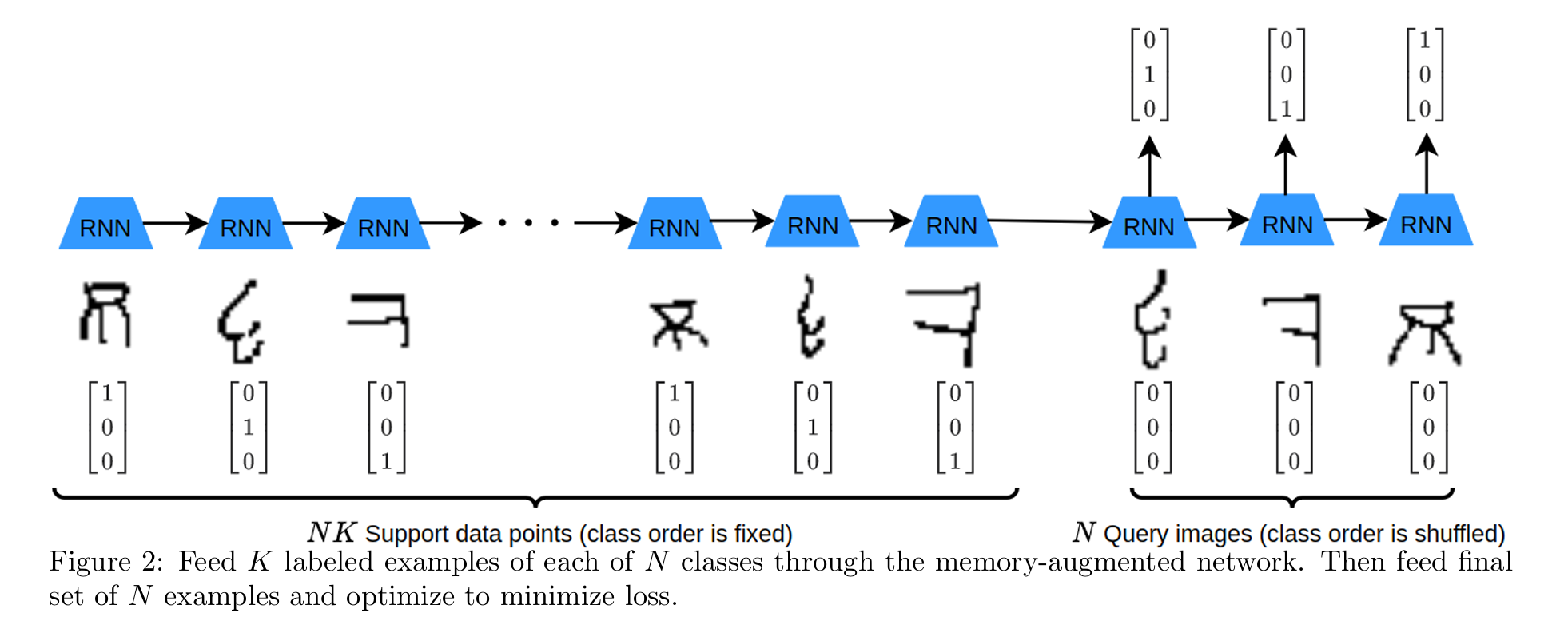
This is the MANN (memory-augmented neural network) architecture:
LSTM
Here are some useful reading materials for understanding LSTM and RNN:
- What is LSTM (Long Short Term Memory)?
- PyTorch Tutorial - RNN & LSTM & GRU
- PyTorch Tutorial - Name Classification Using A RNN
Here’s a nice diagram of LSTM from Understanding LSTM Networks:
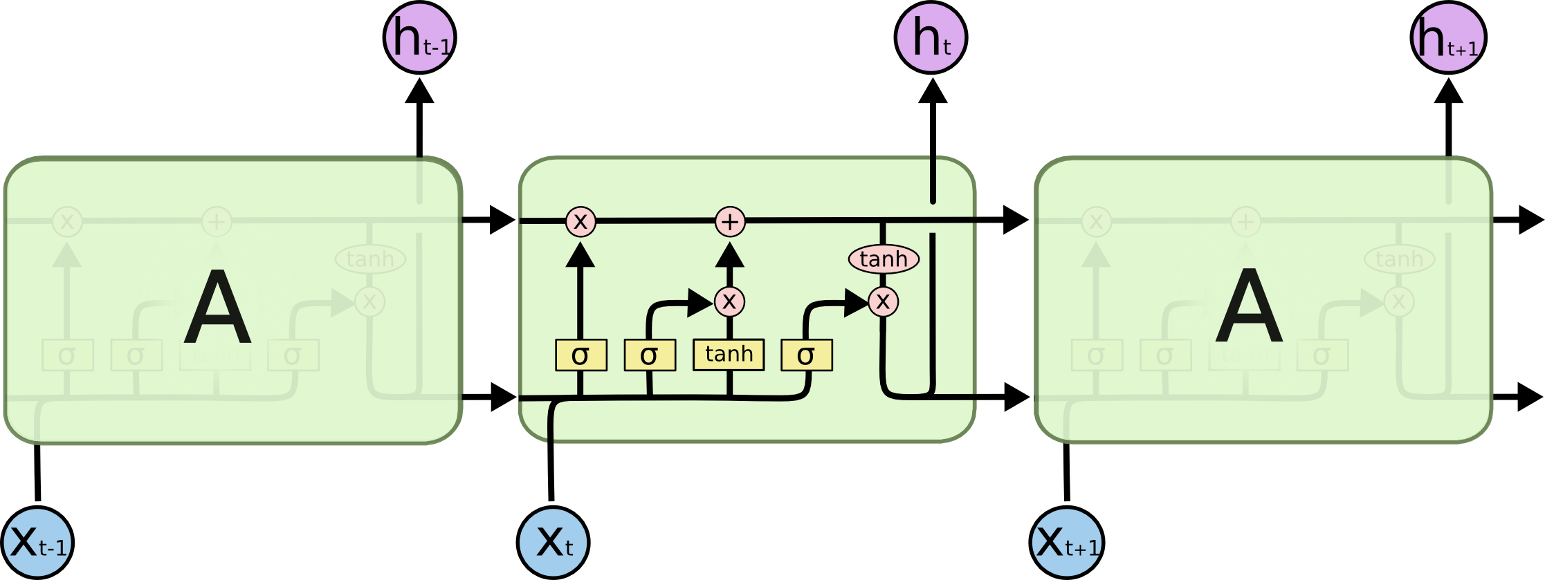
Basically, both GRU and LSTM are type of RNN (Recurrent Neural Network).
I will have a blog that covers the topics in the future.
PyTorch LSTM Module
PyTorch already provides a LSTM module and here’s an example of usage:
import torch
from torch import nn

# Define an LSTM layer with batch_first=True
lstm = nn.LSTM(input_size=10, hidden_size=20, batch_first=True)

# Create a random input tensor with shape (batch_size, seq_len, features)
input_tensor = torch.randn(5, 3, 10)  # (batch_size=5, seq_len=3, features=10)

# Pass the input tensor through the LSTM layer
output, (hn, cn) = lstm(input_tensor)

print(output.shape)  # Output shape: (5, 3, 20)
print(hn.shape)      # Hidden state shape: (1, 5, 20)
print(cn.shape)      # Cell state shape: (1, 5, 20)
Here’s how the MANN architecture is implemented in this assigment:
self.layer1 = torch.nn.LSTM(784 + num_classes, hidden_dim, batch_first=True)
self.layer2 = torch.nn.LSTM(hidden_dim, num_classes, batch_first=True)
Some keypoints:
- By default, PyTorch expects the tensor to have shape
(seq_len, batch_size, features). whenbatch_first = true, it expects tensor to have shape(batch_size, seq_len, features) seq_lenis the sequence lence and in this context, it is theK+1charactersfeaturesin this context is the concatenation of image and label, and its dimension is784 + number of classes(hn, cn)are thehidden stateandcell state, and these are LSTM specific components. We don’t use them in this assignment, we just use theoutput
Implementation
Forward Function
The model inputs are:
imagesarray with shape of[B, K+1, N, 784]labelsarray with shape of[B, K+1, N, N]
I used torch.cate((t1, t2), dim=-1) to concatenate two arrays for the last dimension.
After this operation, the shape becomes [B, K+1, N, 784+N].
I used tensor.view() to reshape the concatenated array to the target dimension, which is [B, (K+1)*N, 784+N].
To see the difference between view() and reshape(), check out reshape() vs view().
Basically, view() creates a new view of the original tensor and is more memory efficient.
Once we have the reshaped input, we just need to pass it to the two LSTM layers:
out, _ = self.layer1(input)
out, _ = self.layer2(out)

# Need to reshape the output to the target output
out = out.view(B, K+1, N, N)
return out
Loss Function
The inputs are:
preds: the output of LSTM, with shape[B, K+1, N, N]labels: the ground truth labels, with shape[B, K+1, N, N]
The output is the cross entropy loss of the predictions and ground truth labels.
Note that the cross_entropy function expects the predictions to have the shape [batch_size, num_classes] and the labels to have the shape [batch_size].
Therefore, we need to reshape the predictions and labels:
- We can get the last N examples with slicing:
preds[:, -1, :, :] - We can reshape the test labels:
test_labels.argmax(dim=-1).reshape(-1)