Introduction
In traditional machine learning, we have a lot of dataset for a specific tasks, while in meta-learning, we have many tasks with small datasets, and the hope is that we can train a model that can learn some fundamental idea from other tasks.
Put it this way: the goal of traditional ML is to optimize the performance of a single task, while the goal of meta-learning is to optimize for adaptability.
In this assignment, we will learn the MAML algorith.
MAML stands for Model-Agnostic Meta-Learning, and it is a very popular algorithm in meta-learning.
In a nutshell, MAML tries to find a parameter vector $\theta$ that allows the model to be quickly adapted to new tasks.
Here’s the image that I got from the XCS330 lecture notes:
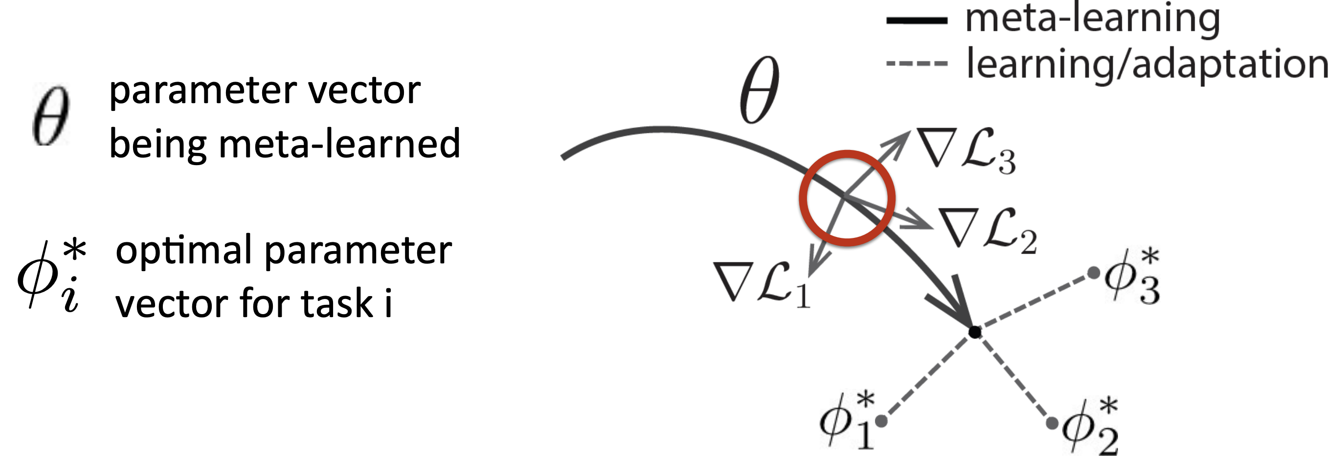
In this assignment, we will need to implement the inner loop and outer loop of the MAML algorithm.
MAML Deep-Dive
Besides the XCS330 lecture notes, I also watched Professor Hung-yi Lee (李宏毅)’s lecture notes on MAML. For those who understand Mandarin Chinese, I highly recommend it. Here’s the link to the first lecture.
In this section, I want to share some notes from the video.
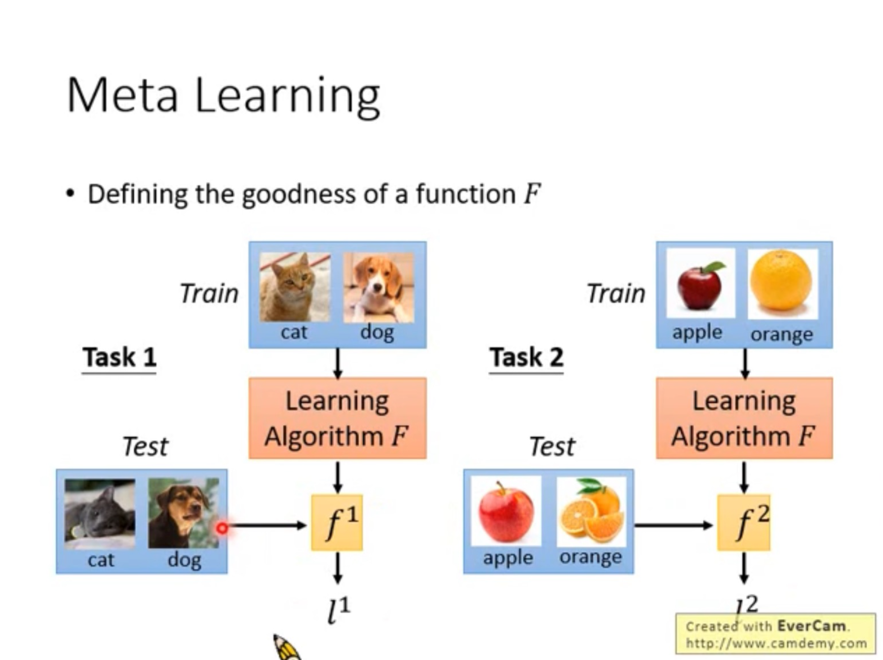
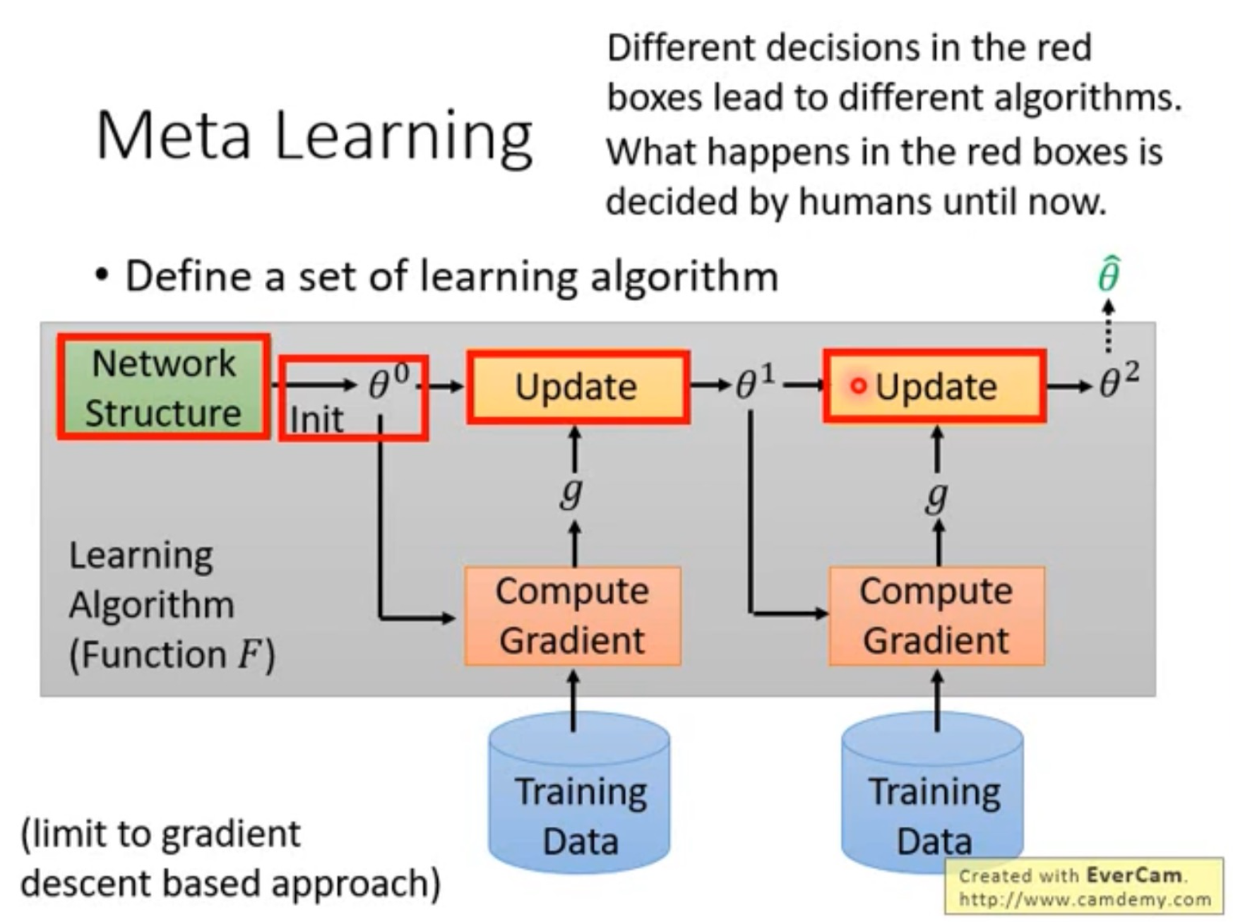
First of all, the goal of MAML is to find a function $F$ such that it can output a mapping function $f$ which can learn new tasks quickly - again, the goal here is the adaptability:
There are two loops in the MAML algorithm:
- inner loop
- outer loop
Inner Loop
In the inner loop, MAML focuses on task-specific training. In this step, MAML uses the support set data to update the paramters $\phi$, and this is very similar to the traditional ML. Here’s the definition of the loss function in this step:
$$ \newcommand{\dataset}{\mathcal{D}} \begin{equation} \mathcal{L}(\phi, \dataset_i) = \frac{1}{\lvert \dataset_i \rvert} \sum_{(x^j, y^j) \in \dataset_i} -\log p_\phi (y = y^j \mid x^j) \end{equation} $$
Outer Loop
In the outer loop, MAML focuses on meta-learning. In this step, MAML optimizes $\theta$ on the query data so that the model is optimized for adaptability.
Note that in the inner loop, the model optimizes for task-specific parameters $\phi$ while here the model optimizes for the meta-learning parameters $\theta$. (Note: $\phi$ is a copy of $\theta$ at the beginning of each inner loop).
Implementation
In this section, I will talk about some implementation details. The notes here are very specific to the assignment and pytorch. Feel free to skip it since the context here is lost for most readers.
Understand requires_grad
To implement the inner loop, I need to understand torch.autograd, and I read this tutorial. Here are some notes that I took from it.
Background
Neural networks are a collection of functions executed on some input data.
Training NN happens in two steps:
- forward propagation: $y = f(x)$
- backward propagation: NN adjusts its parameters by traversing backwards from the output, and use the error and the derivatives to update the params.
Example
Let’s say we have a function $Q = 3a^3-b^2$, where $Q$ is the loss, and $a$ and $b$ are parameters.
import torch

a = torch.tensor([2., 3.], requires_grad=True)
b = torch.tensor([6., 4.], requires_grad=True)

Q = 3*a**3 - b**2
When we call .backward() on Q, autograd calculates these gradients and stores them in the tensors’ .grad attribute.
print(9*a**2 == a.grad)
print(-2*b == b.grad)
I highly recommend these YouTube videos:
- How do computational graphs and autograd in PyTorch work
- PyTorch Autograd Explained - In-depth Tutorial
Understand autograd.grad()
I got these answers from Google (copy-paste):
In PyTorch, torch.autograd.grad() is a function used for computing gradients. It calculates the sum of gradients of specified output tensors with respect to input tensors.

Unlike tensor.backward(), which accumulates gradients into the .grad attribute of leaf tensors, torch.autograd.grad() returns the gradients directly without modifying the .grad attributes.

This provides more flexibility when computing gradients for specific tensors or when needing to prevent accumulation.
Here’s the example (copy-paste):
import torch

# Example usage
x = torch.tensor(2.0, requires_grad=True)
y = torch.tensor(3.0, requires_grad=True)
z = x * y

gradients = torch.autograd.grad(z, [x, y])
print(gradients)  # Output: (tensor(3.), tensor(2.))