In the 3rd assignment of XCS330, we will implement prototypical neworks (protonets) for few-shots image classification on the Omniglot dataset.
Protonets Algorithm
This is the protonet in a nutshell, and the example comes from the assignment:
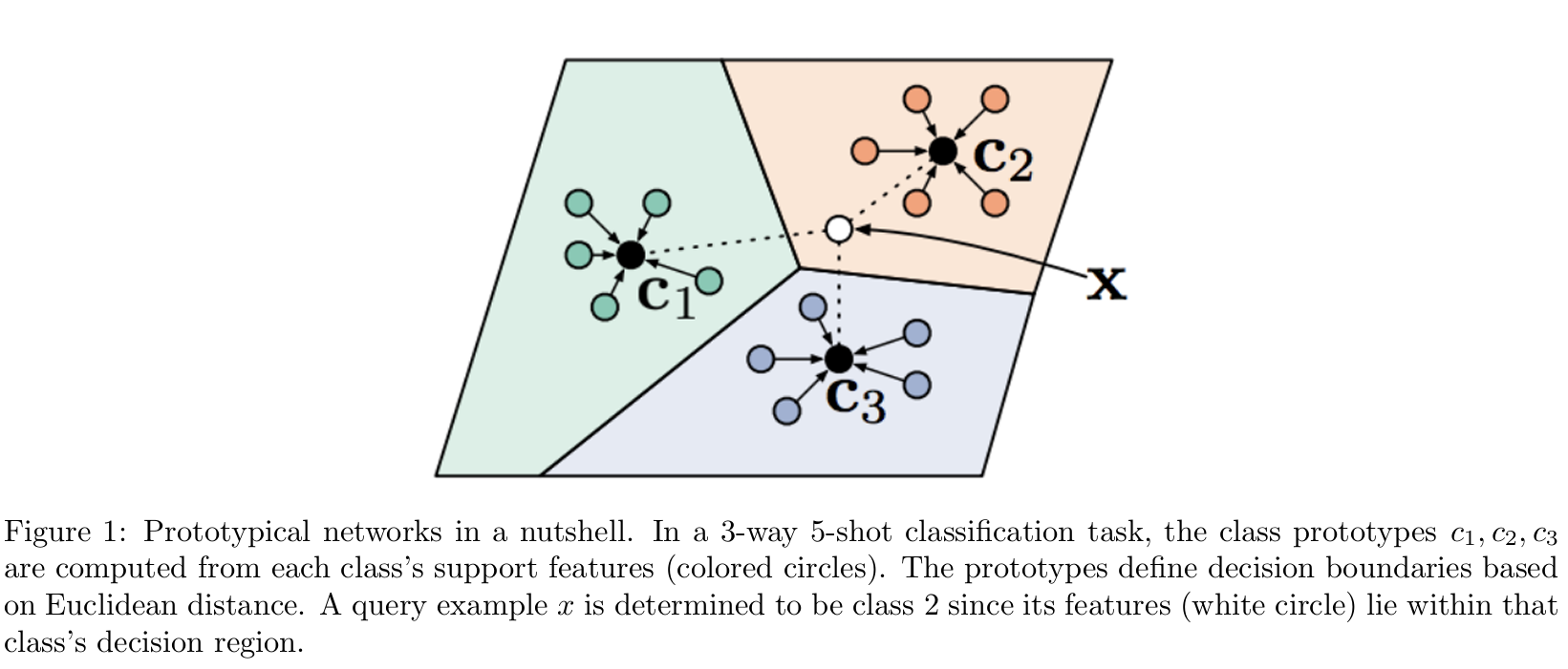
In this example, we compute three class prototypes c1, c2, c3 from the support features. The decision boundaries are computed using Euclidean distance. When there’s a new query, we can determine which class it belongs to.
Implement ProtoNet._step Method
The first coding task is to implement the ProtoNet._step method, which computest the accuracy metrics.
The input of this function is a task batch, and the output is the mean ProtoNet loss over the batch shape.
Here’s the instruction:
- compute the prototypes
- compute the protonet loss
- use cross entropy to compute the classification loss
- use util.score to compute accuracies
Let’s divide and conquer these tasks.
Input & Output Shape
I ran the basic test with >python grader.py 1b-0-basic and got the following shapes:
# print(images_support.shape)
torch.Size([5, 1, 28, 28])

# print(labels_support.shape)
torch.Size([5])

# print(images_query.shape)
torch.Size([75, 1, 28, 28])

# print(labels_query.shape)
torch.Size([75])
These shapes are determined by the setUp() function:
self.dataloader_train = omniglot.get_omniglot_dataloader(
    split='train',
    batch_size=16,
    num_way=5,
    num_support=1,
    num_query=15,
    num_tasks_per_epoch=240000
)
Here we got 5 classes, with 1 support set and 15 query sets.
Understand ProtoNet
The network definition is in the __init__() function:
class ProtoNetNetwork(nn.Module):
    """Container for ProtoNet weights and image-to-latent computation."""

    def __init__(self, device):
        """Inits ProtoNetNetwork.

        The network consists of four convolutional blocks, each comprising a
        convolution layer, a batch normalization layer, ReLU activation, and 2x2
        max pooling for downsampling. There is an additional flattening
        operation at the end.

        Note that unlike conventional use, batch normalization is always done
        with batch statistics, regardless of whether we are training or
        evaluating. This technically makes meta-learning transductive, as
        opposed to inductive.

        Args:
            device (str): device to be used
        """
        super().__init__()
        layers = []
        in_channels = NUM_INPUT_CHANNELS
        for _ in range(NUM_CONV_LAYERS):
            layers.append(
                nn.Conv2d(
                    in_channels,
                    NUM_HIDDEN_CHANNELS,
                    (KERNEL_SIZE, KERNEL_SIZE),
                    padding='same'
                )
            )
            layers.append(nn.BatchNorm2d(NUM_HIDDEN_CHANNELS))
            layers.append(nn.ReLU())
            layers.append(nn.MaxPool2d(2))
            in_channels = NUM_HIDDEN_CHANNELS
        layers.append(nn.Flatten())
        self._layers = nn.Sequential(*layers)
        self.to(device)
The docs string is self explanatory.
The neural network takes an image as the input, and outputs a feature representation of that image, and that is: shape (num_images, latents)
Compute Protoypes
This is the math representation of a prototype:
$$ c_n = \frac{1}{K} \sum_{(x,y) \in \mathcal{D}^\mathrm{tr}i: y=n} f\theta(x) $$
We use a mapping function $f_\theta(.)$ to map the images to features.
We then iterate over the K examples in the training dataset to calculate the prototype.
Here’s the implementation of it:
prototypes = []
for i in range(labels_support.max() + 1):
    # get the latent of the i-th class
    latents = self._network(images_support[labels_support == i])
    # take the mean of the latents
    prototypes.append(latents.mean(dim=0))
Basically, we want to find all the images for the i-th class, use the network to get the latents, and then calculate the mean of it. Note that (dim=0) is needed, otherwise, the mean() function returns the average over all numbers.
Compute Loss
Once we have the prototype, we then use squared Euclidean distance to measure the difference.
$$ d(f_\theta(x), c_n) = | f_\theta(x) - c_n |_2^2 $$
We define the logits as the negative distance -d, which makes sense, because the closer the latent vectors are, the similar the images are.
Finally, we use the cross entropy function to calculate the loss.
Note that, we use support set to compute the prototypes, but we use the query set to calculate the loss.
Also note that, the input tensor for the cross_entropy function is the logits nor the prbabilities! During the implementation, I first applied the softmax function to get the prbabilities and then use it as the input, which is wrong!
torch.nn.functional.cross_entropy

Parameters:
- input: predicted unnormalized logits
- target: ground truth class indicies or class probabilities

Shape:
- input: (N, C)
- target: (N)

where:
C = number of classes
N = batch size
Example
Again, let’s use the unit tests as the example. Assume we have 5 prototypes and each prototype c is a latent vector:
$$ \begin{bmatrix} \begin{bmatrix} c1 \end{bmatrix}\ \begin{bmatrix} c2 \end{bmatrix}\ …\ \begin{bmatrix} c5 \end{bmatrix} \end{bmatrix} $$
And let’s assume we have 75 query images:
$$ \begin{bmatrix} \begin{bmatrix} image 1 \end{bmatrix}\ \begin{bmatrix} image 2 \end{bmatrix}\ …\ \begin{bmatrix} image 75 \end{bmatrix} \end{bmatrix} $$
The first step is to use the model $f_\theta(.)$ to map the images to features. After the mapping, we have:
$$ \begin{bmatrix} \begin{bmatrix} latent 1 \end{bmatrix}\ \begin{bmatrix} latent 2 \end{bmatrix}\ …\ \begin{bmatrix} latent 75 \end{bmatrix} \end{bmatrix} $$
Let’s focus on the operation with all latents, but one prototype.
All latents here means query_latents and it has a shape of [75, d].
One prototype here is c1 and it has a shape of [d].
When we do (query_latents - prototype1)**2, we got:
$$ \begin{bmatrix} \begin{bmatrix} || latent 1 - c1 ||^2 \end{bmatrix}\ \begin{bmatrix} || latent 2 - c1 ||^2 \end{bmatrix}\ …\ \begin{bmatrix} || latent 75 - c1 ||^2 \end{bmatrix} \end{bmatrix} $$
Once we have the diff square, we can then use torch.sum(a, dim=1) to calculate the squared Euclidean distance:
$$ \begin{bmatrix} \begin{bmatrix} d_1 \end{bmatrix}\ \begin{bmatrix} d_2 \end{bmatrix}\ …\ \begin{bmatrix} d_{75} \end{bmatrix} \end{bmatrix} $$
Finally we use the torch.stack([], dim=1) function to extend the distance along the column axis.
Torch.no_grad()
We also need to use torch.no_grad() to compute prototypes.